A32: Multi-class Classification Using Logistic Regression
Multi-class classification, one-vs-rest (ovr), and multinomial logistic regression (polytomous or softmax or multinomial logit (mlogit) or the maximum entropy (MaxEnt) classifier or the conditional maximum entropy model)
This article is a part of “Data Science from Scratch — Can I to I Can”, A Lecture Notes Book Series. (click here to get your copy today!)
💐Click here to FOLLOW ME for new content 💐
⚠️ Benchmark dataset is used for learning purposes.
✅ A Suggestion: Open a new Jupyter notebook and type the code while reading this article, doing is learning, and yes, “PLEASE Read the comment, they are very useful!”
🧘🏻♂️Topics to be covered:
- The dataset, EDA, and preprocessing
- One vs rest
- Multinomial
- Predicted probabilities
- Readings
- Code example
Logistic regression is one of the most popular and widely used classification algorithms and by default, it is limited to a binary class classification problem. However, the logistic regression can be used for multi-class classification as well using its extension like one-vs-rest (ovr) and multinomial.
- In one-vs-rest, the problem is first transformed into multiple binary classification problems, and under the hood, separate binary classifiers are trained for all classes.
- whereas for the multinomial, the solvers learn a true multinomial logistic regression model (4.3.4: Pattern Recognition and Machine Learning by Christopher M. Bishop), and in this case, the probability estimates should be better calibrated than one-vs-rest. The cross-entropy error/loss function (eq: 4.108 in 4.3.4) natively support multi-class classification problem. — maximum likelihood estimation
Let’s work with a multi-class classification problem using both of the above-mentioned extensions in logistic regression.
import pandas as pd; import numpy as np
import matplotlib.pyplot as plt
import seaborn as sns
sns.set_style(‘whitegrid’) # just optional!
%matplotlib inline#Setting display format to retina in matplotlib to see better quality images.
from IPython.display import set_matplotlib_formats
set_matplotlib_formats(‘retina’)# Lines below are just to ignore warnings
import warnings; warnings.filterwarnings(‘ignore’)
We will be working with a very famous the iris dataset. It is on classifying three flower types based on some given features.
1. The dataset, EDA, and preprocessing
iris_df=pd.read_csv(“https://raw.githubusercontent.com/junaidqazi/DataSets_Practice_ScienceAcademy/master/Iris.csv")
Id column is extra, we can drop this column. We can also convert Species column to categorical codes. Let's do this!

All good, there is no missing data. Species and target columns are actually the same but different types. We just need one of them and will handle it while separating the features and a target.
The target column has a balanced class distribution, 50 observations from each class!
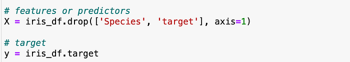
Separating features and the target
Let’s separate features and the target in X and y respectively.
Feature scaling
This must be a known step for all of you now, we have scaled the features in our previous lectures as well!
#scaler = StandardScaler()# Let's try MiMaxScaler here!
scaler = MinMaxScaler()
X = scaler.fit_transform(X)# Try both MinMaxScaler and StandardScaler, and compare the performance of your models!
Machine Learning
As we know it’s a multi-class classification problem, let’s explicitly compare ovr one-vs-rest and multinomialapproaches.
<shift-tab> to explore the documentation, see what happen if multi_class='auto' and the problem is multi-class.
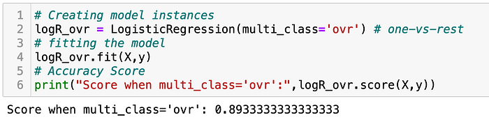
2. One-vs-rest
So, recall what we learned at the beginning on one-vs-rest, and let's get it done!
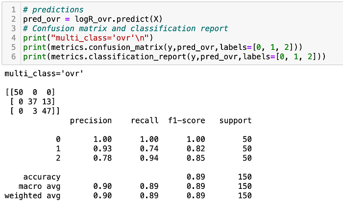
Let’s look at the confusion matrix and classification reports to explore a little more on the performance of our models.
3. Multinomial
Let’s try multinomial for the same data and compare the results!
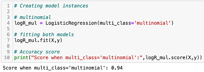
Well, as expected, the multinomial is giving better accuracy!
Let’s look at the confusion matrix and classification reports to explore a little more the performance of our models.

🧘🏻♂️Little more on multi-class logistic regression (optional read)🧘🏻♂
👉 Multiclass logistic regression is also known as polytomous logistic regression, multinomial logistic regression, softmax regression, multinomial logit (mlogit), the maximum entropy (MaxEnt) classifier, and the conditional maximum entropy model.
👉 The multinomial logistic regression assumes that the odds of preferring a certain class over other/s do not depend on the presence or absence of other irrelevant alternatives. So the model choices are independent of irrelevant alternatives, which is a core hypothesis in relational choice theory. A typical example in predicting animal from images that we can think of, the relative probabilities of predicting a horse or cat don’t not change if another choice of lion is added as an additional possibility.
- if class_0 is a preferred choice over class_1 from the given choices set {class_0, class_1}, then adding another choice of class_3 must not make the class_1 preferable on class_0 from the new set of choices {class_0, class_1, class_2}.
This allows the choice of K alternatives to be modeled as a set of K-1 independent binary choices, in which one alternative is chosen as a “pivot” and the other K-1 compared against it, one at a time.
4. Predicted probabilities
We can get the predicted probabilities as well, which is simple.
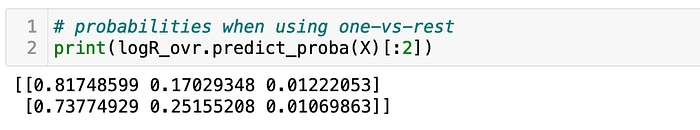
OVR
logR_ovr is our trained model using one-vs-rest, let get the probabilities of the predictions instead of predicted class.
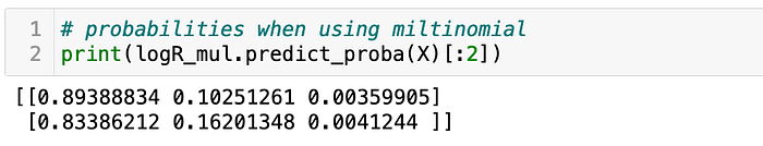
Multinomial
logR_mul is the one we are training using multinomial logistic regression, let’s get the probabilities!
>>ROC-Curve for multi-class classification problem! >> We can create the ROC curve for our multi-class problem, however, we need to treat the problem as a binary class and we will have multiple curves. ROC is only possible for binary classification problems. The provided links in the reading will be useful if you want to create a ROC curve for a multi-class classification problem:
5. Readings
- Multinomial Logistic Regression a nice read
- MLR
- Multinomial Logistic Regression Models
- Great explanation on cross-entropy
- Getting ROC plot for multi-class using scikit-learn
- Precision-recall plot for multi-class problem using scikit-learn
- For Multi-class classification — Gaussian process classification (GPC) based on Laplace approximation
- Partial Dependence Plots
- Individual Conditional Expectation plots
- Scikit-learn: Partial Dependence and Individual Conditional Expectation plots
All goos so far, at this stage, we know how to work with multi-class classification problems. It might be good to have some coding practice as well, the example below will be greatly helpful. Spend some time, code yourself and try to understand the working. Please read the comments that are given with the code, they will be extremely helpful!
6. Code example
Well, this is just for your practice, copy the code below in your own Jupyter notebook and play around to tune a multinomial logistic regression. Please read the given comments and understand the code well.
# Tune regularization for multinomial logistic regression
import time
import numpy as np
from sklearn.datasets import make_classification,make_blobs
from sklearn.model_selection import cross_val_score,RepeatedStratifiedKFold
from sklearn.linear_model import LogisticRegression
import matplotlib.pyplot as plt
start_time=time.time()# get the dataset
def the_dataset():
“””
Creating dataset with 10000 samples and 130 features
using make_classification(). Classes are 5!!!
“””
#X,y=make_blobs(n_samples=100000,centers=5,n_features=5,
# random_state=101,cluster_std=3)
X,y=make_classification(n_samples=10000, n_features=130,n_informative=60,
n_redundant=40,random_state=101,n_classes=5,class_sep=1.5)
# change n_sample=100000 in make_classification
print(“Data (X, y) is created…..”)
return X, y# get a list of models to evaluate
def the_models():
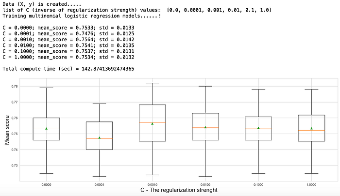
C=[0.0,0.0001,0.001,0.01,0.1,1.0]
print(“list of C (inverse of regularization strength) values: “, C)
print(“Training multinomial logistic regression models……!”)
print()
models=dict()
for p in C:
# create name for model
key=’%.4f’ % p
#print(key)
# turn off penalty in some cases
if p==0.0:
# no penalty in this case
# lbfgs is a default algorithm for parameter optimization and uses limited memory
# based on Broyden–Fletcher–Goldfarb–Shanno (bfgs) algorithm
models[key]=LogisticRegression(multi_class=’multinomial’,
solver=’lbfgs’,penalty=’none’)
else:
models[key]=LogisticRegression(multi_class=’multinomial’,
solver=’lbfgs’,
penalty=’l2',C=p)
return models# evaluate a give model using cross-validation
def model_eval(model,X,y):
“””
this is the docstring for this function.
“””
# define the evaluation procedure
cv = RepeatedStratifiedKFold(n_splits=10, n_repeats=5, random_state=101) # creating instance
# Stratification is the process of dividing members of the population into
# homogeneous subgroups before sampling.
# evaluate the model
scores = cross_val_score(model, X, y, scoring=’accuracy’, cv=cv, n_jobs=-1)
return scores# define dataset
X, y = the_dataset()
# get the models to evaluate
models = the_models()
# evaluate the models and store results
results, names = list(), list()
for name, model in models.items():
# evaluate the model and collect the scores
scores = model_eval(model, X, y)
# store the results
results.append(scores)
names.append(name)
# summarize progress along the way
print(“C = {}; mean_score = {}; std = {} “.format(
name,round(np.mean(scores),4),round(np.std(scores),4)))
print(“\nTotal compute time (sec) = {}”.format(time.time() — start_time))# plot model performance for comparison
plt.figure(figsize=(18,6))
plt.xlabel(“C — The regularization strenght”, fontsize=18);plt.ylabel(“Mean score”, fontsize=18)
plt.boxplot(results, labels=names, showmeans=True);
Please note, this lecture covers several concepts from the previous lecture, such as standardization, model training, ROC-Curve, etc. if you are following me from the first lecture on Data Science from Scratch, everything should be fine, if not and you need some clarification, please explore previous lectures.
Our main focus is to bring more and more professionals into the field of data science so that they can achieve their full potential.
Good luck!
💐Click here to FOLLOW ME for new content 💐
🌹Keep practicing to brush-up & add new skills🌹
✅🌹💐💐💐🌹✅ Please clap and share >> you can help us to reach to someone who is struggling to learn these concepts.✅🌹💐💐💐🌹✅
Good luck!
See you in the next lecture on “A33: Handling imbalanced classes in the dataset!”.
Note: This complete course, including video lectures and Jupyter notebooks, is available on the following links:
Dr. Junaid Qazi is a subject matter specialist, data science & machine learning consultant, and team builder. He is a professional development coach, mentor, author, technical writer, and invited speaker. Dr. Qazi can be reached for consulting projects, technical writing and/or professional development trainings via LinkedIn.

More content at plainenglish.io. Sign up for our free weekly newsletter. Get exclusive access to writing opportunities and advice in our community Discord.